
Deep learning is the family of machine learning methods that train multilayer neural networks to learn hierarchical representations from data. It is the engine behind modern computer vision, speech recognition, and large-scale language modeling—but it is not automatically the best tool for every tabular, low-data, or heavily regulated decision problem. This guide explains what depth buys you, how modality-specific systems are trained and transferred, how production train and serve stacks diverge, and where deep models fail in ways classical methods usually do not.
The goal is an engineering mental model: when deep learning is justified, how to train and evaluate it, and how to operate it without confusing notebook accuracy for product reliability. Unit-level pedagogy—activations, loss algebra, and architecture family inductive biases—lives primarily in the neural networks guide; this page owns representation learning at system scale.
What deep learning is (and is not) relative to classical ML
Deep learning earns its name from depth in the computational graph: many parameterized stages between input and prediction. Historically, the practical breakthrough was not the idea of multilayer networks alone, but the combination of better initialization and normalization practices, abundant labeled and unlabeled data, and accelerator hardware that made large-scale gradient descent routine. Once those pieces aligned, end-to-end learned features displaced many hand-engineered pipelines in perception and sequence modeling.
Classical machine learning often relies on hand-designed features plus a comparatively shallow predictor: linear models, kernel methods, boosted trees, and related estimators. Deep learning shifts most of the feature construction into the model. Layers compose nonlinear transforms so that useful structure—edges, motifs, tokens, spectro-temporal patterns—emerges from optimization rather than from a fixed feature recipe.
That shift has a cost. Deep models usually need more data, more compute, and more careful validation than a well-tuned gradient-boosted tree on a clean tabular problem. They also concentrate risk in the training pipeline: silent data bugs, unstable optimization, and train/serve skew can produce confident errors that look fluent in demos.
Deep learning is therefore best understood as a bet on representation learning: that hierarchical parameters can absorb structure that would be expensive or impossible to engineer by hand. It is not a synonym for artificial intelligence, not a requirement for every predictive system, and not a license to skip problem framing, metrics, or operational controls.
Representation learning: why depth helps
Representations are intermediate vectors (or tensors) that make downstream prediction easier. An embedding of an image, utterance, or document is valuable when distances and directions in that space track task-relevant similarity. Deep stacks build those embeddings by successive refinement. The same idea underpins transfer: a representation trained for one broad objective can initialize another.
Empirically, depth interacts with width, data, and regularization. Extremely deep stacks without residual pathways historically suffered from vanishing or exploding gradients; modern residual and normalization patterns mitigate that. Still, adding layers is not free. Each layer increases compute, memory for activations during training, and the chance of fitting noise. Capacity should be justified by validation curves and slice behavior, not by parameter fashion.
A useful way to think about depth is compositional reuse. Early layers detect local, reusable patterns; later layers recombine those patterns into task-specific abstractions. In vision, that progression often looks like edges → textures → parts → objects. In speech and language, local acoustic or lexical cues combine into longer-range structure. The hypothesis is not that deeper is always better; it is that depth expands the set of functions that can be learned efficiently from raw or lightly processed inputs.
Formally, supervised deep learning usually minimizes an empirical risk over parameters θ. Given examples (xᵢ, yᵢ) and a loss ℓ, training seeks
θ̂ ≈ arg min_θ (1/n) Σᵢ ℓ(f_θ(xᵢ), yᵢ) + Ω(θ)
where f_θ is a deep network and Ω is optional regularization. Overfitting appears when the empirical risk on training data falls while risk on the deployment distribution rises. Depth increases capacity; capacity without the right data, inductive bias, and regularization produces memorization rather than transferable structure.
Depth helps when the target function is hierarchical and the data distribution supports learning those hierarchies. Depth hurts when the signal is sparse, the labels are noisy relative to capacity, or the important features are already explicit in a small engineered table—cases where classical models often win on calibration, data efficiency, and auditability.
Building blocks in brief (defer full unit pedagogy to neural-networks)
Every deep model is still a neural network: stacked linear transforms, nonlinearities, and a training procedure that estimates gradients through the computational graph. Weights, activations, attention blocks, residual connections, and normalization layers are the parts. The neural networks guide is the right place for unit definitions, activation choices, and architecture-family pedagogy.
What matters here is the systems consequence of those parts. Residuals and normalization make very deep stacks trainable. Convolution and attention encode different assumptions about locality and global mixing. Parameter count interacts with data volume and compute budget. Backpropagation is the standard algorithm for computing gradients; frameworks automate it, but engineers still own shape bugs, mixed-precision numerics, and frozen-subgraph mistakes that break learning silently.
Keep the division of labor sharp: this page routes you to neural networks for “what is a layer,” and keeps ownership of “how deep systems are trained, transferred, evaluated, and served across modalities.”
Supervised deep learning workflow at production scale
Label quality deserves explicit budget. Deep models punish ambiguous ontologies. If annotators disagree on edge cases, the model will learn an unstable average and fail on the same edges in production. Invest in gold sets, adjudication, and periodic ontology review. For detection and segmentation, annotation protocols (box tightness, crowd rules, ignore regions) are part of the model definition.
Experiment discipline prevents false progress. Fix seeds where possible, log data hashes, and compare against a frozen baseline every cycle. When using pretrained weights, record the exact checkpoint source and license. Promotion should require a written eval against the previous production candidate under identical harness code.
A production supervised workflow is larger than a training script. It includes problem framing, data contracts, label ontology, split discipline, training jobs, evaluation gates, packaging, deployment, and monitoring. At scale, the expensive parts are often data and iteration latency—not the elegance of the architecture diagram.
Start with the decision the model will support. Define the output type (class, box, mask, sequence, scalar), the cost of errors, and the slices that must not fail silently. Then design labels and splits that respect time, site, device, customer, or other leakage axes. Only then choose an architecture and training recipe.
Training at production scale usually means distributed data loading, checkpointing, experiment tracking, and reproducible configs. Teams that skip lineage invent archaeology later: nobody can explain which data version produced the weights in production. A minimum operating bar is: dataset version, code version, hyperparameters, hardware target, and eval report attached to every candidate that might be promoted.
Self-supervised pretraining and transfer ladders
Self-supervision reframes the data problem. Instead of paying for labels on every pretraining example, the objective invents targets: predict masked content, discriminate augmented views, or model sequences autoregressively. The representation becomes generally useful if the pretext task forces the network to capture structure that correlates with downstream needs. That correlation is not guaranteed—pretext design and data mix matter.
Negative transfer is real. Adapting a pretrained model into a mismatched domain can degrade a strong baseline. Detect it with controls: compare against training from scratch or against a simpler model on the same labeled set. If adaptation hurts the primary slices, stop climbing the ladder.
Transfer learning is one of deep learning’s practical advantages. Instead of training every task from random initialization, teams pretrain on a broad objective, then adapt to a narrower one. Self-supervised pretraining removes the need for exhaustive labels during the expensive representation-learning phase by defining pretext tasks from the data itself: masked prediction, contrastive agreement, next-token prediction, and related objectives.
Adapter vs full fine-tune vs continued pretrain
After pretraining, adaptation choices form a ladder. A linear probe or shallow head tests whether the frozen representation already contains the signal. Parameter-efficient adapters and low-rank updates change a small subset of weights and are often enough for moderate domain shift. Full fine-tuning updates most or all parameters and can fit harder shifts at higher risk of catastrophic forgetting and higher compute cost. Continued pretraining on domain text or images sits between general pretraining and task fine-tuning when the domain distribution differs sharply from the original corpus.
| Adaptation method | What changes | Typical fit | Main risks |
|---|---|---|---|
| Linear probe / shallow head | New head only | Strong pretrained features; quick baseline | Underfits large domain shift |
| Adapters / LoRA-style updates | Small parameter subsets | Many enterprise customizations | Capacity limits; bad rank/hyperparameters |
| Full fine-tune | Most/all weights | Hard shifts with enough labeled data | Forgetting; higher cost; harder rollback |
| Continued pretrain then task tune | Broad domain adaptation first | Domain language/vision far from pretrain data | Contamination; long jobs; eval complexity |
The right rung is empirical. Promote with held-out and slice metrics, not with the story that “we fine-tuned, so it must be better.” For procedure detail on adaptation recipes, see fine-tuning; this section owns the transfer ladder as a deep-learning systems pattern.
Architectures by modality: vision, language, speech, tabular caution
Multimodal systems compose modality encoders and fusion modules. Fusion can be early, mid, or late; each choice changes what joint reasoning is possible and what fails under missing modalities. Deep learning makes fusion learnable, but evaluation must include modality dropout and asymmetric noise. When generation enters the picture—images, audio, or text—route detailed generative mechanics to the generative and modality guides; keep this page focused on learned hierarchical encoders and shared training practice.
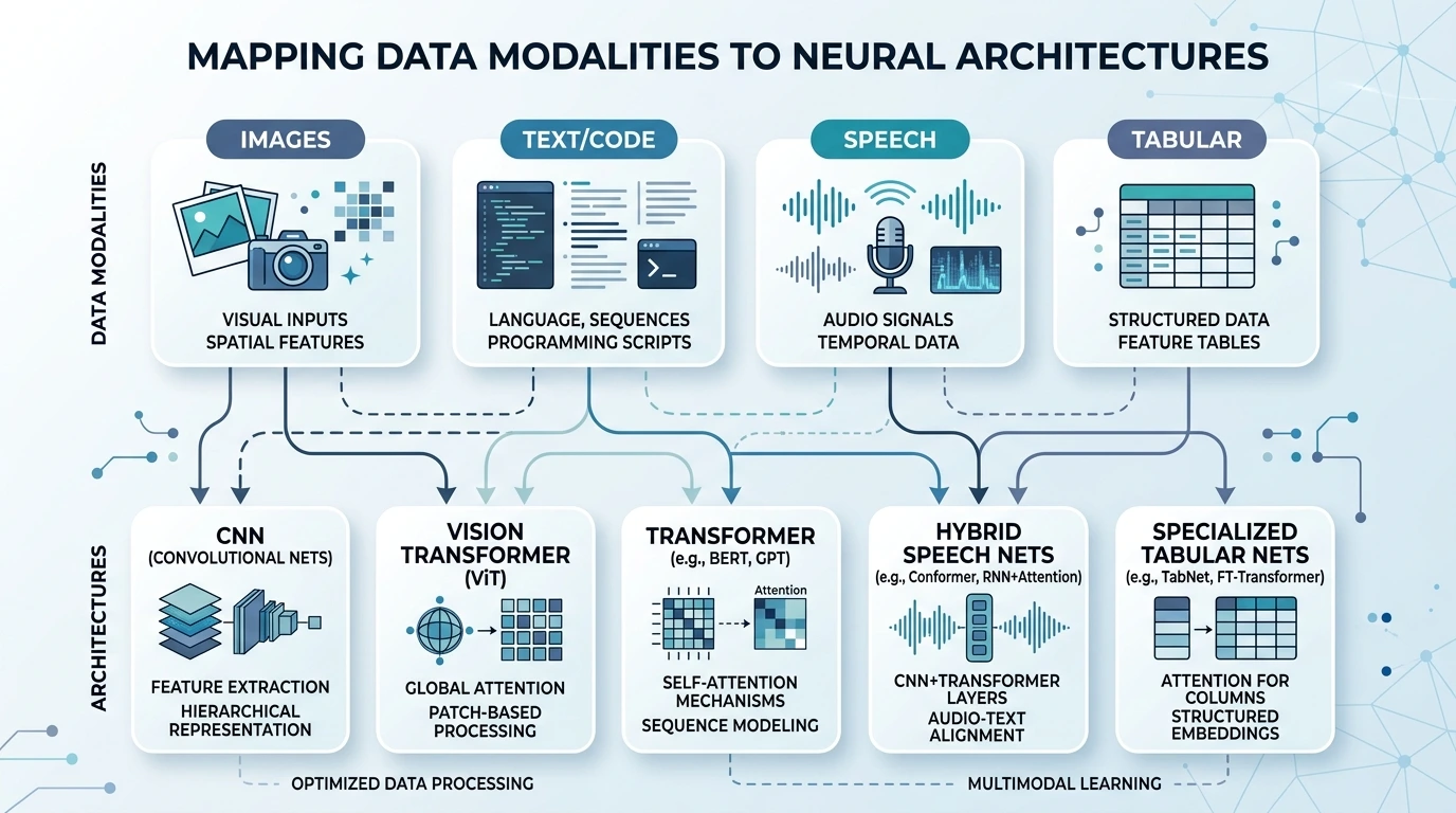
Inductive bias remains a first-class design lever. Convolution privileges locality and weight sharing. Attention privileges flexible routing at quadratic cost in sequence length unless approximated. Recurrence privileges ordered state but parallelizes poorly. Graph networks privilege relational structure. Choosing among them is choosing which assumptions you are willing to bake in before seeing infinite data.
Architecture choice should follow data geometry. Images have local spatial statistics; language has discrete tokens and long-range dependencies; speech is a noisy temporal signal; tables are often heterogeneous and sample-inefficient for pure deep nets.
CNN vs ViT vs hybrid for a given data geometry
In vision, convolutional networks encode translation-friendly local filters and remain strong when data is limited or when inductive bias matters. Vision transformers treat image patches more like tokens and can excel at scale with enough data and regularization. Hybrids borrow both. For detection, segmentation, and video, the surrounding system—FPN-style necks, tracking heads, temporal sampling—often matters as much as the backbone brand. Deep coverage of vision tasks and metrics belongs in computer vision; here the point is modality routing.
For language, transformer stacks dominate modern large-scale modeling. This page will not become a language-model internals or serving encyclopedia—those topics belong in dedicated large language model and generative AI guides. The deep-learning claim is narrower: sequence models learn contextual representations that transfer across tasks when pretraining and adaptation are done carefully.
Speech systems combine convolutional, recurrent, and transformer components depending on streaming constraints and acoustic conditions; see speech and voice AI for task pipelines. Tabular data deserves caution: when features are already informative and n is modest, tree ensembles frequently outperform deep nets on accuracy, calibration, and training cost. Deep tabular models can win in multimodal settings (table + text + image) or at very large scale, but “deep by default” is a common enterprise mistake.
Optimization realities: learning rates, instability, and scaling heuristics
Learning-rate selection is still one of the highest-leverage knobs. Too high and training diverges or oscillates; too low and you waste budget while appearing “stable.” Range tests, warmup, and schedule plots are cheap relative to full training runs. Adaptive methods (Adam-family) are common defaults for transformers; SGD with momentum remains competitive in many vision settings. The optimizer is part of the recipe that must be locked for fair comparisons.
Regularization intersects optimization: weight decay, dropout, stochastic depth, label smoothing, and data augmentation all change the effective objective. Turning every knob at once makes ablations impossible. Change one family of controls at a time when diagnosing under- or overfitting.
Reproducibility deserves skepticism. Nondeterministic GPU kernels, data loader races, and distributed all-reduce ordering can create run-to-run variance. For high-stakes launches, quantify that variance with repeated seeds before celebrating a one-off win.
Deep training is constrained optimization under noisy gradients. Learning-rate schedules, batch size, momentum/adaptive methods, gradient clipping, and initialization interact. Instability shows up as loss spikes, NaNs in mixed precision, attention mask bugs, or data pipeline stalls that look like “the model diverged.”
Useful heuristics exist, but they are heuristics: larger batches often want adjusted learning rates; warmup can stabilize early transformer training; clipping bounds pathological steps; cosine or step decays are common. None of these replaces slice-aware evaluation. Scaling laws and compute-optimal training literature motivate how loss improves with data, parameters, and compute—but production teams still need cost ceilings, latency targets, and diminishing-return analysis for their own distribution.
Optimization ownership in deep learning also includes distributed training failure modes: stragglers, inconsistent sharding, and checkpoint corruption. If your bottleneck is interconnect or storage rather than algorithm choice, the next guide in the stack is infrastructure—not another architecture paper.
Data-centric work for deep models
Long-tail classes dominate many deep-learning failures. Macro metrics hide them. Build dashboards for rare but critical categories and sample them into eval sets deliberately. Active learning and hard-example mining can help, but they can also overfit the mining loop if not carefully gated.
Feedback loops appear when model outputs influence future training data—content ranking, moderation, and fraud being typical. Deep models can accelerate those loops. Document whether training data includes model-influenced samples and prefer counterfactual or holdout policies when possible.
Deep models amplify data problems because they have the capacity to fit them. Duplicate examples, label leakage across splits, silent class imbalance, ontology drift, and sensor changes all become model behavior. Data-centric work means treating datasets as versioned products: documentation, sampling policy, adjudication rules, and quality metrics.
For vision and speech, collection conditions are part of the model. Camera mounts, codecs, microphones, and preprocessing must be specified. For language, contamination between train and eval can manufacture fake progress. Deduplication, license constraints, and PII handling are not side quests; they determine whether a model can be shipped.
Synthetic data and augmentation can help, but only when they preserve label semantics. Aggressive augmentation that changes the decision boundary teaches the wrong invariance. Prefer augmentation ablations with slice metrics over folklore checklists.
Robustness, distribution shift, and calibration
Shift comes in flavors: covariate shift, label shift, and concept drift. Deep models may need different remedies for each. Importance weighting and recalibration help some label-shift cases; representation alignment and augmentation help some covariate cases; concept drift often demands fresh labels and retraining triggers. Monitoring should name which shift you suspect.
Out-of-distribution detection is imperfect but useful as a tripwire. Scores based on softmax confidence alone are often weak. Distance-in-representation methods and dedicated OOD detectors can help route uncertain cases to humans or safer fallbacks. Fallbacks are product features, not apologies.
Deployment distributions drift. Lighting changes, user language shifts, fraudsters adapt, and hospitals use different scanners. Deep models can be brittle under shift while remaining confident. Robustness work includes stress sets, data augmentation matched to real shift, domain adaptation, and monitoring that watches slices—not only global averages.
Calibration matters whenever downstream systems treat scores as probabilities. A model with strong discrimination can still be miscalibrated. Temperature scaling and related post-hoc methods help in some settings; they do not fix shortcut learning. If the model relies on spurious cues, better calibration merely makes the wrong reason look precise.
Shortcut learning is a deep-learning-specific operational hazard: high capacity finds any correlate, including watermark artifacts, hospital tokens, or dataset indices. Adversarial evaluation and slice design are how you discover those correlates before customers do.
Train systems versus serve systems
Batching policy illustrates the train/serve split. Training batches maximize throughput and gradient quality under memory limits. Serving batches (or continuous batching) exist to improve accelerator utilization without violating latency SLOs. A model that looks cheap at batch 128 in a bench can be expensive at batch 1 online. Measure the serving shape you will actually run.
Model packaging should include preprocessing, vocabulary/image ops, and postprocessing as versioned artifacts. Shipping bare weights invites silent skew. Prefer immutable release candidates: weights + config + preprocessing commit + eval report as one unit.
Training optimizes parameters. Serving optimizes latency, cost, reliability, and change control. Conflating the two produces fragile launches: a research checkpoint bolted to an API without preprocessing parity, batching policy, or rollback.
| Concern | Train systems | Serve systems |
|---|---|---|
| Objective | Minimize training/validation risk | Meet latency/availability/cost SLOs |
| Data path | Epochs over sharded datasets | Single request or micro-batch online |
| Hardware bent | Throughput across accelerators | Tail latency and utilization |
| Failure mode | Divergent loss, bad checkpoint | Timeouts, OOM, silent quality drop |
| Change control | Experiment tracking | Canary, rollback, config freeze |
Parity bugs are classic: different resize kernels, text-normalization versions, normalization constants, or text normalization between train and serve. Build a shared preprocessing library and test it. Canary deployments with slice dashboards catch many failures that offline eval misses. Accelerator vendors such as NVIDIA and frameworks such as PyTorch shape the practical train/serve toolchain, but tools do not replace parity tests.
Evaluation that matches deployment decisions
Cost-sensitive thresholds belong in the eval harness. If false negatives cost ten times false positives, report the operating point that reflects that ratio—not the threshold that maximizes a convenient F1 on a balanced set. For ranking and retrieval heads used with deep encoders, report recall at practical cutoffs and calibrate expectations for long-tail queries.
Human evaluation remains necessary for many perception and generative-adjacent outputs. Design rubrics, measure rater agreement, and separate rater drift from model drift. Automated metrics are accelerants, not replacements, when the decision is subjective or safety-critical.
Leaderboard metrics are not product metrics. Choose metrics that encode the decision: precision/recall at a threshold, calibration under shift, worst-slice recall, latency at p95, and cost per successful prediction. For generative heads attached to deep models, add task-specific quality and safety checks—without turning this page into an LLM evaluation manual.
Offline eval needs representative and adversarial sets. Online eval needs guardrails: shadow traffic, capped canaries, and kill switches. A promotion packet should answer: what improved, what regressed, which slices were checked, what the rollback path is, and who owns incidents.
Statistical humility helps. Small gains on noisy eval sets are not launches. Multiple comparisons across dozens of experiments inflate false discoveries. Pre-register the primary metric when stakes are high.
Failure modes unique to deep models
Another distinctive failure is “benchmark illusion”: a deep model climbs a public leaderboard that shares train-test contamination or that fails to represent deployment hardware and demographics. Private, contamination-controlled eval sets are part of serious deep-learning practice. So is testing under the compression and batching settings used in production, because accuracy after quantization is the accuracy customers experience.
Dependency failure matters too. Downstream services that treat model scores as truth will cascade errors. Contract tests between the model service and callers—schema, score semantics, timeout behavior—prevent deep models from becoming un-owned magic.
Deep learning fails in characteristic ways:
- Train/serve skew: preprocessing or data path differences flip outcomes.
- Spurious correlation: high capacity latches onto shortcuts.
- Catastrophic forgetting: fine-tuning erases prior skills.
- Distributed data bugs: silent shard imbalance or label map mismatches.
- Overconfident errors: especially with generative or poorly calibrated heads.
- Numerics: mixed precision overflow/underflow and nondeterministic kernels that complicate debugging.
Incident response should include dataset diffs, config diffs, and slice dashboards—not only “retrain with a new backbone.” Many production incidents are data or parity incidents wearing an architecture costume.
Hardware and efficiency constraints (quantization, distillation)
Memory walls dominate many modern architectures. Attention and large activations can make training throughput memory-bound before compute-bound. Activation checkpointing trades compute for memory; ZeRO-style optimizer sharding trades communication patterns for larger models. Engineers should know which wall they are hitting before buying more GPUs as a first response.
On the inference side, graph compilation, kernel fusion, speculative techniques for sequence models, and caching of repeated prefixes can dwarf minor architecture tweaks. Efficiency work is deep-learning work when the model family and representation stack create the bottleneck profile.
Deep models are constrained by memory bandwidth, accelerator availability, and energy cost as much as by algorithms. Inference budgets force compression: quantization, pruning, distillation, distillation-to-smaller architectures, and caching. Quantization reduces numeric precision to shrink memory and improve throughput; distillation trains a smaller student to mimic a larger teacher. Both can preserve average metrics while damaging tail slices—so evaluate the slices you care about after compression.
Training efficiency matters too: gradient checkpointing, mixed precision, compiled graphs, and better data pipelines often yield more than a fashionable architecture change. When the limiter is cluster design, interconnect, or serving runtime, escalate to AI infrastructure and model hosting concerns rather than burying them here.
When not to use deep learning
Regulatory or contractual settings that demand transparent feature contributions may favor generalized linear models or monotonic constrained models. Deep explanations (saliency, attributions) can help debugging but rarely satisfy the same standards as inherently interpretable forms. Choose the model class that matches the accountability regime you actually have.
Finally, do not use deep learning as organizational avoidance. If the hard problem is messy definitions, missing owners, or unavailable labels, a deeper net will not invent a product strategy. Fix the problem framing first.
Skip deep learning when a simpler model meets the metric, when labeled data are scarce relative to needed robustness, when hard interpretability constraints dominate, or when tabular structure already encodes the signal. Prefer classical baselines early; they are not a retreat, they are a control group.
Also skip deep learning when the organization cannot operate it: no eval harness, no monitoring, no rollback, no owner for data quality. A shallow model with an honest metric beats an unowned deep system that cannot be diagnosed.
Multimodal products sometimes need deep components for perception and a classical or rules layer for decisions. Hybrid systems are normal. The deep-learning mistake is insisting that one end-to-end net must own every business rule.
DL-specific governance: memorization and bias amplification
Memorization risk grows with model capacity and with unique or repeated sensitive strings in training data. Mitigations include deduplication, filtering, differential privacy training in specialized settings, output filtering, and strict access control to weights and training corpora. None is perfect; layered controls beat single silver bullets.
Bias amplification shows up when training data reflect historical skew and the model’s capacity makes that skew sharper in predictions. Measure group and slice errors, examine annotation pipelines for skewed labels, and decide whether the correct intervention is data work, constrained optimization, thresholding policy, or not deploying to that decision. Technical metrics must connect to an accountable decision owner.
Deep models can memorize rare training examples and amplify biases present in data. Memorization creates privacy and security exposure; bias amplification creates uneven error rates across groups and contexts. Governance for deep learning therefore includes dataset documentation, access controls, retention limits, eval for sensitive slices, and processes for model change.
This is not a substitute for a full ethics or regulatory program—those belong in dedicated guides—but deep learning adds concrete technical failure modes that governance must track: extraction risk from large models, unequal slice performance after fine-tuning, and silent regressions when data pipelines change. Treat model cards and datasheets as operational artifacts, not marketing PDFs.
Boundaries with neighboring Knowledge guides
Deep learning sits inside machine learning and overlaps neural networks, generative modeling, and modality systems. Use this page for hierarchical representation learning and deep train/serve practice. Use neural networks for units and architecture families. Use modality guides for task metrics. Use LLM and generative guides for token-centric and cross-modality generation stacks. Keeping those boundaries is how the Knowledge library stays non-duplicative.
References and further reading
Authoritative starting points (verify details against the original publications and current documentation):
- LeCun, Y., Bengio, Y., & Hinton, G. (2015). Deep learning. Nature, 521, 436–444.
- Goodfellow, I., Bengio, Y., & Courville, A. (2016). Deep Learning. MIT Press.
- He, K., et al. (2016). Deep Residual Learning for Image Recognition. CVPR.
- Vaswani, A., et al. (2017). Attention Is All You Need. NeurIPS.
- Dosovitskiy, A., et al. (2021). An Image Is Worth 16×16 Words: Transformers for Image Recognition at Scale. ICLR.
- PyTorch Autograd documentation — official framework docs for automatic differentiation.
- NIST AI Risk Management Framework for governance context around AI systems.