
A neural network is a parameterized function built from interconnected computational units that transform inputs through weighted combinations and nonlinearities. Multilayer perceptrons, convolutional nets, recurrent nets, and transformers are different wiring patterns over that substrate. This guide explains what a network computes, how forward and backward passes work, how architecture families encode inductive bias, and where neural function classes hit hard limits.
If you need representation-learning systems practice, adaptation workflows at product scale, or production training and inference operations, use the deep learning guide. This page owns the mechanics shared by large language models: units, graphs, losses, backpropagation, topologies, and architectural choice—not deep-learning systems operations. Frameworks such as PyTorch implement autograd for these graphs; the math does not depend on any single vendor.
Parameterized functions: what a network computes
It helps to write the prediction as ŷ = f(x; θ) and to treat θ as a single flattened vector only for optimization talk—while remembering that real implementations keep structured tensors for efficiency. Reshaping for optimizers must preserve the exact correspondence between gradient entries and parameters. Silent misalignment here trains the wrong object.
Identifiability is limited: many different θ can realize nearly identical functions, especially with permutations of hidden units. That is why comparing raw weight values across runs is usually meaningless, while comparing predictions and representation probes can be informative.
At root, a neural network is a function f_θ mapping an input x to an output ŷ, where θ collects trainable parameters—weights, biases, and related tensors. Training searches for θ that make ŷ useful under a chosen loss. Inference evaluates f_θ with θ fixed. That split between choosing parameters and applying them is the entire training/inference distinction at the model level.
Three questions should stay separate. First: what function class can the architecture represent? Second: how do gradient methods search that class? Third: which inductive biases did you hard-wire before seeing data? Neural nets are powerful because differentiable composition yields flexible classes, not because individual units are magical.
A feedforward net is a directed acyclic computational graph. Recurrent designs introduce cycles in time; training unfolds them into feedforward graphs over sequences. Graphs make shapes and dependencies explicit. If you cannot name the tensors and ops on the path from x to ŷ, you cannot debug learning.
Every parameter participates in concrete ops: matrix multiplication, convolution, embedding lookup, normalization, attention. The forward pass is a program; the backward pass is that program’s derivative. Frameworks automate derivatives; they do not invent correct graphs. Masking errors, accidental detaches, and silent broadcasts still produce scalar losses with wrong meaning.
Two nets can share loss and data yet compute different functions because their graphs differ. Architecture is a claim about which functions are easy to represent and optimize. Choosing a family is choosing a prior over functions.
Units, layers, and nonlinearities
A useful teaching limit is the single neuron classifier: σ(wᵀx + b) with a logistic σ implements a linear decision boundary in x-space. Nonlinear boundaries require either nonlinear features or multilayer nonlinear compositions. Hidden layers synthesize features; the output layer maps them to task targets.
Dead ReLU units—stuck with nonpositive pre-activations and zero derivatives—reduce effective capacity. High learning rates and poor init increase that risk. Leaky or parametric variants mitigate but do not remove the need for sound scale control.
A standard fully connected unit computes an affine map then a nonlinearity: σ(wᵀh + b). A dense layer applies many units in parallel: ĥ = σ(Wh + b). The weight matrix mixes features; the bias shifts thresholds; the activation injects nonlinearity.
Without nonlinearities, depth collapses. A stack hℓ+1 = Wℓhℓ + bℓ telescopes to one affine map. Nonlinearities break that collapse and make depth representationally meaningful. “More layers” without σ is not more power.
Activations and gradient health
ReLU and variants are piecewise linear and sparse on the negative side, with simple derivatives that avoid the classic sigmoid saturation regime for positive pre-activations. Sigmoid and tanh are smooth and bounded, but large |z| drives σ′(z)→0, which multiplies into vanishing updates for earlier parameters. Activation choice is therefore both a representational bias and a numerical bias.
Layers are interfaces: they group parameters and define the representation passed onward. Residual links reparameterize a block toward h ↦ h + F(h), giving identity paths that empirically stabilize deep stacks for both forward signal and backward gradients.
Initialization sets the starting scale of weights so activations neither explode nor die at step zero. Good initializers match activation families. Biases are often started near zero unless a known prior exists. Treat init as part of the architecture contract, not an afterthought.
Forward propagation
Batching changes the leading tensor dimension but not the mathematical map applied to each example (except when layers explicitly couple batch elements, as in batch normalization). Document which layers are batch-dependent. Forward propagation in train mode may include noise sources; eval mode should disable them.
For convolutional and attention layers, forward propagation includes reshape/transpose patterns that are easy to get almost right. Almost-right shapes often fail only on certain sequence lengths or image sizes—test multiple shapes.
Forward propagation evaluates the graph from inputs to outputs. For an MLP:
a₀ = x; zℓ = Wℓ aℓ−1 + bℓ; aℓ = σℓ(zℓ)
until the final layer emits logits or predictions. Values aℓ are activations; zℓ are pre-activations. Training retains intermediates needed for backward (or recomputes them under checkpointing). Inference may drop unused tensors.
Forward-pass failures are common and boring: transposed matrices, unintended broadcasting, double softmax, train-mode normalization during evaluation, or off-by-one sequence masks. Before interpreting a loss curve, verify shapes on a single batch and check a tiny hand example where the correct output is known.
Stochastic layers (dropout) behave differently in train versus eval. Forward propagation must use the mode that matches the contract. Mixing modes is a frequent source of “it trains but eval looks random” bugs.
Losses as decision contracts
Multi-class cross-entropy from logits z and label class c can be written −z_c + log Σ_j exp(z_j). That form shows why subtracting the max logit before the exponential is a numerical stability trick, not a modeling change. Implementing loss from hand-built probabilities is a common source of underflow bugs.
When labels are uncertain, losses may use soft targets or explicit noise models. That is still a contract change: you are no longer claiming a single hard y. Keep the contract matched to how annotators actually labeled.
A loss ℓ(ŷ, y) is a contract stating what counts as error. Classification commonly uses cross-entropy from logits; regression uses squared or absolute error; ranking and structured prediction need specialized surrogates. Softmax combined with cross-entropy is usually computed in a log-sum-exp stable form from logits rather than materializing probabilities first.
The objective is typically empirical risk plus optional regularization:
J(θ) = (1/n) Σᵢ ℓ(f_θ(xᵢ), yᵢ) + Ω(θ)
Ω may include weight decay. Changing ℓ changes the surface you descend. A model can minimize a convenient surrogate while failing the real decision costs. Publish the operating point (threshold, top-k, calibration need) alongside the loss.
Loss geometry affects gradient scale. Large residuals under squared error punch hard; confident wrong class probabilities under cross-entropy also punch hard. When steps explode or stall, ask whether the loss-plus-activation pair is producing pathological gradient magnitudes before inventing new layers.
Backpropagation and automatic differentiation
Mini-batch gradients average (or sum) contributions across examples. Scaling conventions differ across frameworks and papers; mismatching them effectively rescales the learning rate. When porting recipes, check whether the loss is mean- or sum-reduced.
Second-order methods exist but are less common at large scale than first-order adaptive methods. Curvature diagnostics (gradient noise scale, Hessian-vector products in research settings) can explain stubborn plateaus, yet most practical debugging still starts with first-order gradient health.
Teacher-forcing in sequence models and truncated backprop through time are deliberate graph truncations. They bias gradients to shorter dependencies in exchange for tractability. Know when your backward graph is truncated on purpose.
Backpropagation computes ∂J/∂θ by reverse-mode application of the chain rule. Forward builds intermediates and the scalar loss; backward pushes sensitivities from the loss toward parameters. For y=a(b(c(x))), local derivatives multiply along the path. On tensors, reverse mode efficiently yields gradients for many parameters from one scalar objective.
Locally, for ĥ=σ(Wh+b), the gradient w.r.t. W depends on upstream h and downstream ∂J/∂ĥ, filtered by σ′(z). Backprop is bookkeeping that assembles local Jacobians into a global parameter gradient. That bookkeeping is the learning algorithm’s backbone.
Gradient descent and stochastic mini-batch variants update θ ← θ − η∇_θJ, optionally with momentum or adaptive rescaling. Backprop supplies ∇; the optimizer consumes it. A flat loss with near-zero gradients suggests saturation, tiny init, dead ReLUs, or a learning rate that is too small. A violently unstable loss suggests the opposite scale problem—or data labels that are garbage.
Credit assignment through depth and through time is the hard part. Vanishing gradients shrink early updates; exploding gradients blow up steps. Gated recurrence, residual pathways, normalization, and gradient clipping are tools for keeping flow usable. They are not alternatives to a correct objective.
Automatic differentiation implements reverse mode for you. It will happily differentiate the wrong graph. Stop-gradient ops, detached tensors, and incorrect masks change which parameters move. Always ask: “which edges are live in the backward graph?”
Capacity, generalization, and the bias-variance tension
Double descent phenomena and benign overfitting results show that classical U-shaped risk curves are incomplete for some modern nets. They do not authorize skipping test sets. If anything, they increase the need for contamination-aware evaluation because memorization can coexist with good average test scores on easy distributions.
Effective capacity depends on optimization and regularization, not only on parameter count. Early stopping and augmentation can make a large net behave smaller. Report the training procedure when you claim a capacity result.
Capacity describes how flexible the function class is. Width, depth, and freer connectivity generally increase capacity. Insufficient capacity underfits; excess capacity can interpolate noise when data are scarce or labels are noisy. Modern overparameterized regimes complicate cartoon U-curves, yet held-out evaluation remains non-negotiable.
Overfitting is the pattern where training loss improves while unseen loss worsens or stalls. Neural nets memorize readily because they can. Architectural bias, data diversity, regularization, and early stopping are the primary countermeasures at the model level.
Evaluate on splits that respect leakage structure—time, entity, device, site. If validation shares contamination with training, you are measuring memorization skill. Capacity arguments without honest splits are not science.
Multilayer perceptrons and tabular caution
Feature scaling matters more for dense nets than for tree ensembles. Unnormalized continuous features can dominate initial logits and distort learning. Standardize or otherwise condition inputs unless the architecture explicitly absorbs scale.
Embeddings for categorical variables turn MLPs into mixed symbolic-numeric models. Embedding dimension is a capacity knob with overfitting risk on rare categories. That is still neural-network mechanics—not a detour into product recommender systems.
An MLP stacks dense nonlinear layers. Theory says multilayer nets with nonlinearities can approximate broad function classes under mild conditions; practice says MLPs are a strong default when inputs are already feature vectors without spatial or sequential layout.
On heterogeneous tabular problems with modest sample size, gradient-boosted trees frequently match or beat MLPs on accuracy and calibration with less fuss. Trees exploit axis-aligned structure efficiently; dense nets must learn it. Use MLPs when differentiability end-to-end matters; do not crown them default kings of spreadsheets.
Width and depth are not interchangeable knobs. Deep thin MLPs often need residuals or normalization to train; wide shallow nets spend parameters on mixing at fewer abstraction levels. Compare them with the same budget and the same splits.
Convolutional inductive bias for spatial structure
Equivariance and invariance language clarifies CNN behavior: weight sharing encourages translation-equivariant features; pooling promotes approximate invariance to small shifts. Neither property is absolute under padding tricks, boundary effects, or aggressive downsampling.
1×1 convolutions are channel mixers without spatial neighborhood mixing—useful as dimension adapters inside larger CNN blocks. Depthwise separable patterns factor spatial and channel mixing for parameter efficiency. These are architectural factorizations, not magical accuracy guarantees.
Convolutional networks replace dense global mixing with local filters shared across positions. The prior matches images and other grids: local correlation and translational reuse. Parameter count scales with kernel size and channels rather than full spatial resolution times features.
Stride, padding, and dilation control coverage; stacked layers grow receptive fields. Downsampling via pooling or strided convolution trades resolution for field of view and compute. The inductive claim is locality plus weight sharing—not a guarantee of vision product success.
For task families, metrics, and deployment of vision systems, see computer vision. Here the point is architectural: if your dependence structure is non-local, convolution’s prior can be harmful. Attention-based vision models relax locality and shift burden onto data scale and regularization.
Sequence models: RNN legacy versus transformer parallelism
In an LSTM-style cell, gates typically regulate input, forget, and output pathways around a cell state that can carry information with fewer repeated multiplications than a vanilla RNN state. The qualitative win is improved long-range gradient flow; the qualitative cost is more parameters and more ops per step.
Bidirectional RNNs combine forward and backward states for offline sequence labeling. They are invalid for true causal streaming. Architecture choice must respect the information availability of the deployment setting—even though this page is not a serving manual.
Recurrent networks carry a state through time: ht=Φ(ht−1, xt). That inductive bias fits ordered sequences and streaming updates. Vanilla recurrence multiplies many Jacobians through time, which invites vanishing and exploding gradients on long dependencies.
Gated architectures (LSTM/GRU families) introduce learned gates that modulate information flow, improving the odds that gradients traverse long sequences. Even then, training remains sequential along length, limiting parallelism.
Transformers substitute content-based attention for much of that recurrence, allowing parallel computation across positions during training. The cost moves to attention memory and compute, often growing steeply with length unless approximated, and to the need for explicit positional structure. Pick the bias that matches sequence statistics and hardware constraints.
Attention, positions, and context windows
Self-attention builds Q, K, V from the same sequence; cross-attention draws K, V from another stream. Both are the same mathematical primitive with different sources. Residual connections and normalization around attention blocks are part of making deep attention stacks trainable.
Sparse and linearized attention variants change the inductive bias and complexity class by restricting which positions may interact. When you adopt them, you are changing the architecture’s dependency prior, not merely “speeding up the same model.”
Scaled dot-product attention routes information by similarity:
Attention(Q, K, V) = softmax((QKᵀ)/√dk) V
Queries probe keys; resulting weights mix values. The √dk scale counters growth of dot products with dimension that would otherwise sharpen softmax and damage gradients. Multi-head attention repeats the mechanism in parallel subspaces.
Because attention is a function of content-derived Q, K, V, position must be injected—absolute encodings, relative biases, or other schemes. The context window is how much of the sequence can be conditioned on in one forward pass. Larger windows raise memory and can change quality unevenly across distances.
Masks implement rules: causal masks block future positions for autoregression; padding masks block empty slots. A broken mask can reduce loss while leaking illegal context. Treat mask tests as unit tests for the architecture.
Normalization, residuals, and trainability tricks
Pre-norm versus post-norm placement alters training dynamics in deep residual/attention stacks. The difference is empirical and architecture-specific; treat placement as part of the architecture definition you lock for fair comparisons.
Gradient clipping sets a maximum norm or value for updates. It prevents rare huge gradients from destroying training but can hide underlying scale bugs if used as a permanent crutch. Investigate the source of explosions when clipping triggers continuously.
Deep graphs are sensitive to activation scale. Batch normalization, layer normalization, and related methods re-center and re-scale intermediate distributions. Their behavior depends on batch size, axes normalized, and interaction with residuals. A recipe that works in one regime can fail in another.
Residuals, initialization, clipping, and learning-rate warmup are stabilizers. They help optimization traverse a nonconvex landscape; they do not fix wrong labels or a mismatched loss. If gradients look healthy and generalization still fails, return to data and objective before stacking more tricks.
Regularization toolkit (dropout, weight decay, early stop)
Label smoothing softens hard targets and can reduce overconfidence; it changes the loss contract. Stochastic depth and DropPath regularize deep residual stacks by randomly skipping blocks in training. Each technique has a clear mechanism—prefer mechanism-based selection over stacking folklore.
Dropout randomly zeroes units during training to discourage brittle co-adaptation; evaluation uses deterministic scaling. Weight decay penalizes large weights and is often folded into optimizers. Early stopping uses validation signal as a complexity-control brake. Augmentation regularizes only when transforms preserve label semantics.
These mechanisms are not interchangeable. Ablate them. Regularization adjusts effective capacity; it cannot repair an inductive bias that fights the data geometry.
Interpretability without theater
Concept probes train simple classifiers on frozen hidden states to test whether a concept is linearly readable. They measure presence of information under a restricted readout, not that the network “uses” the concept causally. Pair probes with interventions when claims matter.
Most neural nets do not emit human-readable rules. Saliency maps and attribution scores can be debugging hints, not certificates of reasoning. Prefer interventions: remove or corrupt an input region and measure metric change; analyze error slices; examine nearest neighbors in representation space.
When a domain requires inherent transparency, choose a more constrained function class. Post-hoc explanations rarely convert an unconstrained net into something equivalent to a simple audited model.
Mixed precision and numerical failure modes
Loss scaling multiplies the loss before backward to keep small gradients representable in narrow formats, then unscales before applying updates. Incorrect scaling schedules look like mysterious instability. Log whether overflows were detected when diagnosing mixed-precision runs.
Reduced-precision arithmetic improves throughput and memory footprint but shrinks dynamic range. Overflow, underflow, and inadequate loss scaling produce NaNs and sudden divergence. Mixed-precision training keeps sensitive accumulations in wider formats while using narrower formats elsewhere.
Deep computational graphs amplify numerical issues because many multiplications compose. Nondeterministic kernels add run-to-run variance. When debugging, confirm finite activations and gradient norms, then correlate failures with precision settings before redesigning layers. A NaN is frequently a scale problem.
Hard limits of neural function classes
Discrete algorithms with exact invariants—checksums, parsers with hard grammar constraints, safety interlocks—should not be expected to emerge reliably from generic nets without structure. Neuro-symbolic hybrids exist because these limits are real. Knowing the limit is part of competent neural-network engineering.
Neural networks approximate mappings from finite data. They do not automatically acquire causal graphs, symbolic guarantees, or truthful extrapolation beyond support. Hard constraints and safety invariants usually require non-neural checks around the model.
Optimization is typically nonconvex: no general global optimum guarantee; random seeds disagree. Universal approximation theorems do not imply efficient learnability. Finite context, finite precision, and finite samples bound every realized network. Naming these limits prevents category errors about what a trained net “knows.”
Choosing among architecture families
A practical decision sequence: (1) identify grid, sequence, set, graph, or mixed geometry; (2) pick the weakest bias that fits; (3) baseline with default hyperparameters and honest splits; (4) only then add depth/width/attention span. Skipping to a fashionable family without a baseline produces uninterpretable comparisons.
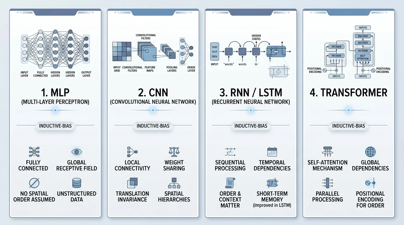
Parameter counts are a weak proxy for cost. Attention and convolution have different compute profiles at equal parameter counts. When constraints are latency or memory on a target device, measure those directly rather than optimizing parameter folklore.
Match family to geometry and constraints:
| Family | Inductive bias | Often fits | Watch-outs |
|---|---|---|---|
| MLP | Dense feature mixing | Tabular/vector inputs; baselines | Ignores spatial/sequential structure unless engineered |
| CNN | Locality + weight sharing | Images/grids | Poor prior if relations are global |
| RNN / gated RNN | Temporal state | Streaming/short-medium sequences | Limited parallelism; long-range strain |
| Transformer | Content-based attention routing | Tokens; flexible long-range mixing | Compute/memory with length; needs positions |
| GNN | Neighborhood aggregation on graphs | Relational data | Oversmoothing; depends on graph quality |
Start with the simplest plausible family, establish a baseline, and escalate complexity only when evaluation demands it. Hybrids are valid when data mix geometries. For broad adaptation workflows, modality product systems, and production training/inference operations, go to deep learning instead of cloning that guide here.
Throughout, prefer graphs, shapes, and inductive-bias arguments over slogans. A neural network earns trust when its function class, training dynamics, and failure modes are understood—not when its diagram looks modern.
Finally, keep evaluation honest at the model level: identical splits, identical preprocessing, and identical loss reduction conventions when comparing architectures. Otherwise you are comparing procedures, not function classes. Lock those controls before declaring a winner.
References and further reading
- Rumelhart, D. E., Hinton, G. E., & Williams, R. J. (1986). Learning representations by back-propagating errors. Nature, 323, 533–536.
- Hochreiter, S., & Schmidhuber, J. (1997). Long short-term memory. Neural Computation, 9(8), 1735–1780.
- Vaswani, A., et al. (2017). Attention Is All You Need. NeurIPS.
- He, K., et al. (2016). Deep Residual Learning for Image Recognition. CVPR.
- Goodfellow, I., Bengio, Y., & Courville, A. (2016). Deep Learning. MIT Press.
- PyTorch Autograd documentation.